Other Transforms

Cosine Transform

Discrete Cosine Transform (DCT)

Uses just $cos$ functions.
We don’t use complex numbers anymore, but we also lose some of the nice properties of the transform (e.g., shift and convolution theorem).
Good tool for compression, not so much for signal analysis.
Coefficients are divided into "DC" (zero frequency) and "AC" (other frequencies) just like with DFT.

Forward DCT:

C (k) = α (k) l = 0 \sum N - 1 f (l) \cdot [cos \frac{( 2 l + 1 ) πk}{2 N}], k = {0, 1, ... N - 1} where α (k) = ⎩ ⎨ ⎧ \frac{1}{N} iff k = 0 \frac{2}{N} iff k \neq = 0

Inverse DCT:

f (l) = k = 0 \sum N - 1 α (k) \cdot C (k) [cos \frac{( 2 l + 1 ) πk}{2 N}], l = {0, 1, ..., N - 1}

Derivation of DCT

Let’s do the following transformation to the original signal $f$ of length $N$ :

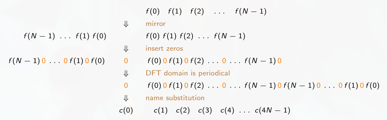Note	The addition of interleaved zeroes is the same as stretching the original signal. $c$ is even (ready for DFT without complex number), has length $4 N$ , and the following is true: $c (2 n) c (2 n + 1) c (4 N - n) = 0 iff 0 \leq n < N = f (n) iff 0 \leq n < N = c (n) iff 0 < n < 2 N$

Apply DFT to $c$ :

$C (k) = j = 0 \sum 4 N - 1 c (j) \cdot e^{- \frac{2 πijk}{4 N}} = /symmetry/ = j = 0 \sum 2 N - 1 c (j) \cdot [e^{\frac{2 πijk}{4 N}} + e^{- \frac{2 πi ( 4 N - j ) k}{4 N}}] = = j = 0 \sum 2 N - 1 c (j) \cdot [e^{- \frac{2 πijk}{4 N}} + e^{\frac{2 πijk}{4 N}}] = /Euler-Moivre eq./ = j = 0 \sum 2 N - 1 c (j) \cdot [(cos \frac{2 πjk}{4 N} - i sin \frac{2 πjk}{4 N}) + (cos \frac{2 πjk}{4 N} + i sin \frac{2 πjk}{4 N})] = = j = 0 \sum 2 N - 1 c (j) \cdot [2 cos \frac{2 πjk}{4 N}] = /split odd and even positions/ = l = 0 \sum N - 1 2 c (2 l) \cdot [cos \frac{2 π 2 l k}{4 N}] + l = 0 \sum N - 1 2 c (2 l + 1) \cdot [cos \frac{2 π ( 2 l + 1 ) k}{4 N}] = /c is 0 at even pos./ = l = 0 \sum N - 1 2 f (l) \cdot [cos \frac{( 2 l + 1 ) πk}{2 N}] (DCT-II)$

Fast discrete cosine transform (F-DCT)

Recombine signal $f$ of length $N$ to get $y$ :

$y (l) = f (2 l) y (N - 1 - l) = f (2 l + 1) (l = 0, 1, ..., N /2 - 1)$
Run FFT on $y$ .
For each $k = 0, 1, ... N - 1$ do:
1. Multiply the k-th Fourier coefficient by factor $e^{- \frac{πik}{2 N}}$ :
  
  $Y^{'} (k) = e^{- \frac{πik}{2 N}} \cdot Y (k)$
2. Get only the real part of each Fourier coefficient and normalize the results:
  
  $C (k) = α (k) \cdot Real [Y^{'} (k)] \cdot N$

Note	The recombination step, which created $y$ , is a clever hack of converting a sequence meant for DCT into something that can be digested by DFT, allowing us to use FFT inside FastDCT.

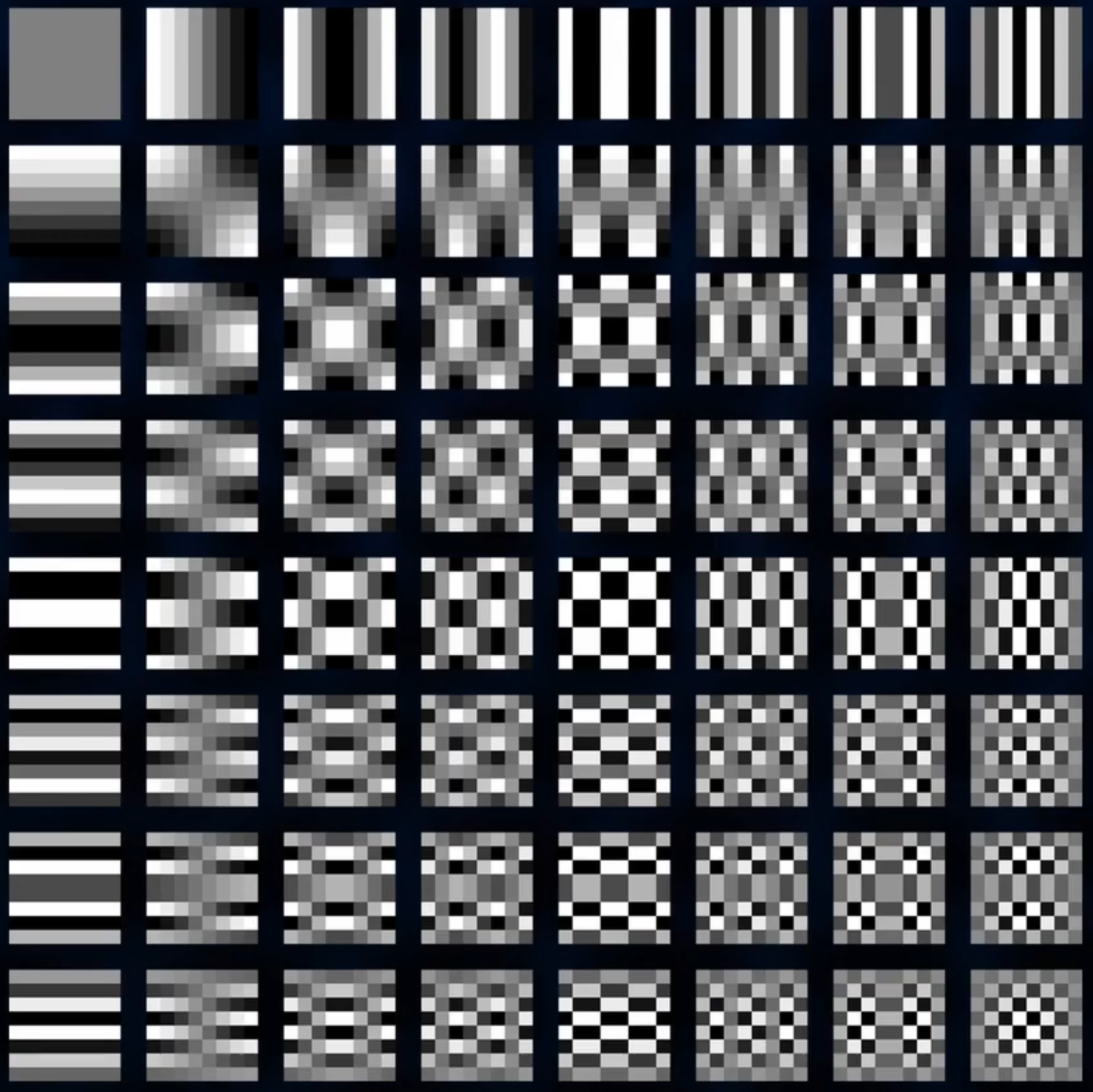
DCT in 2D

Z-transform

Z-transform

It’s a generalization of the (discrete time) Fourier transform. Wheras DTFT projects $f$ on the unit circle in the complex plane, Z-transform uses the whole complex plane. Whereas DTFT can only analyze frequencies that are stable, Z-transform can also handle unstable or exploding signals (e.g., screaching sounds or the whole image turns white or black).

It’s used to check that recursive linear filters don’t blow up to "infinite white" or are unstable.
In optimizing DWT.
Understanding and frequency analysis of linear filters.
Forward Z-tranform converts discrete time series into a continuous signal (Z-plane).
Forward Z-transform applied to discrete signals or linear filters always creats a polynomial with one variable $z$ .

Bilateral forward Z-transform:

F (z) = - \infty \sum \infty f (n) z^{- n} where z \in C

Inverse Z-transform:

If $F (z)$ is a polynomial, that is $F (z) = \sum_{k = - \infty}^{\infty} c_{k} z^{- k}$ , then

f (n) = Z^{- 1} (F (z)) = k = - \infty \sum \infty c_{k} δ (n - k)

Linear recursive filters

The idea is that convolution is computationally expensive ( $O (n^{2})$ ) but if it could be recursive and use already-convolved neighbors as their input, the complexity would be lower ( $O (n lo g n)$ ).

Wavelet Transform

Wavelet transform (WT)

Compared to FT, which captures global frequency information, WT provides temporal information as well.
Uses wavelets — functions with a peak at zero and brief, diminishing oscillations.
- The main idea is to constrain the basis functions in time ("wavelet" = "little wave").
- Parametrized both by frequency and time.
It’s not possible to have perfect information about time and frequency at the same time. WT is in the middle.
A mother wavelet can be any function that satisfies the wavelet constraints.
WT turns a 1D time function $f (t)$ into a 2D function of time and frequency $T (a, b)$ .
We translate the mother wavelet $ψ$ (shift it in time) or scale it (change its frequency).
- Translating $ψ_{b} (t) = ψ (t - b)$
- Scaling $ψ_{a} (t) = ψ (t / a)$
- Scaling and traslating $ψ_{a, b} = ψ (\frac{t - b}{a})$
$ψ_{a, b}$ are the daughter wavelets.
The mother wavelet is complex.
- If it were just real, then when WT would output zero it wouldn’t necessarily mean that there is no wave of the specified frequency because the waves can cancel each other out instead of resonating. We use complex wavelets so that we can take the absolute value of the complex result and avoid this problem.
Time vs frequency trade-off: High-time detail for high frequencies. High-frequency detail for low frequencies.

Continuous Wavelet Transform (CWT)

T (a, b) = \frac{1}{∣ a ∣} \int_{- \infty}^{\infty} f (t) \cdot \overline{ψ_{a, b} (t)} d t

Note	We conjugate $ψ_{a, b}$ because it’s complex and dot product works like that with complex numbers. The $\frac{1}{∣ a ∣}$ is a normalization factor it preserves the "energy" of each stretched daughter wavelet so we treat them equally.

Wavelet constraints

Function $ψ (t)$ is a wavelet if:

Admissability condition: It has zero mean. There is no zero frequency component.

$\int_{- \infty}^{\infty} ψ (t) d t = 0$
Has finite energy. This makes it localized in time.

$\int_{- \infty}^{\infty} ∣ ψ (t) ∣^{2} d t < \infty$

Well-known mother wavelets

Haar — The original wavelet used in DWT. Most educational.
Morlet — Complex exponential ( $e^{i x}$ ) + Gaussian. First wavelet used in CWT.
Daubechies
Shannon
Meyer
Mexican hat
triangular

Obrázek 1. The Haar Wavelet

Discrete Wavelet Transform

Discrete wavelet transform (DWT)

Any WT where the wavelets are discretely sampled. In the following general definition, the original signal $f$ has length $M = 2^{J}$ and $j \in {j_{0}, ..., J - 1}$ is the decomposition level.

All computations are performed with floating point numbers. No complex numbers are used.
One forward step is between two consecutive decomposition levels is just separation of low and high frequencies.
One backward step between two consecutive decomposition levels is just merging of low and high frequencies.
The complete decomposition of a signal can be done step-by-step (i.e., recursively) or all at once (i.e., with a matrix).
The scaling function acts as a "bottom" to the recursion/sub-banding because we need to stop somewhere.
- That being said, we also have to stop once we reach the resolution of the original signal.
The scaling function also shows "trends" in the signal. Thanks to it, we can be sure that we don’t miss any frequencies in the signal. In other words, it fixes the problem which in CWT is addressed by using complex numbers.

Forward DWT:

A_{j_{0}} (k) D_{j} (k) = \frac{1}{M} m = 0 \sum M - 1 f (m) \cdot φ_{j_{0}, k} (m) = \frac{1}{M} m = 0 \sum M - 1 f (m) \cdot ψ_{j, k} (m)

Inverse DWT:

f (m) = \frac{1}{M} k = 0 \sum 2^{j_{0}} - 1 A_{j_{0}} (k) \cdot φ j_{0}, k (m) + \frac{1}{M} j = j_{0} \sum J - 1 k = 0 \sum 2^{j} - 1 D_{j} (k) \cdot ψ_{j, k} (m)

where

$φ$ and $ψ$ — Orthogonal scaling and wavelet functions respectively.
$A_{j_{0}}$ — Scaling coefficients, approximations for low frequencies (low = in the $j_{0}$ sub-band).
$D_{j}$ — Wavelet coefficients, details for high frequencies (high = in the $j$ sub-band).
$k \in {0, 1, ..., 2^{j} - 1}$

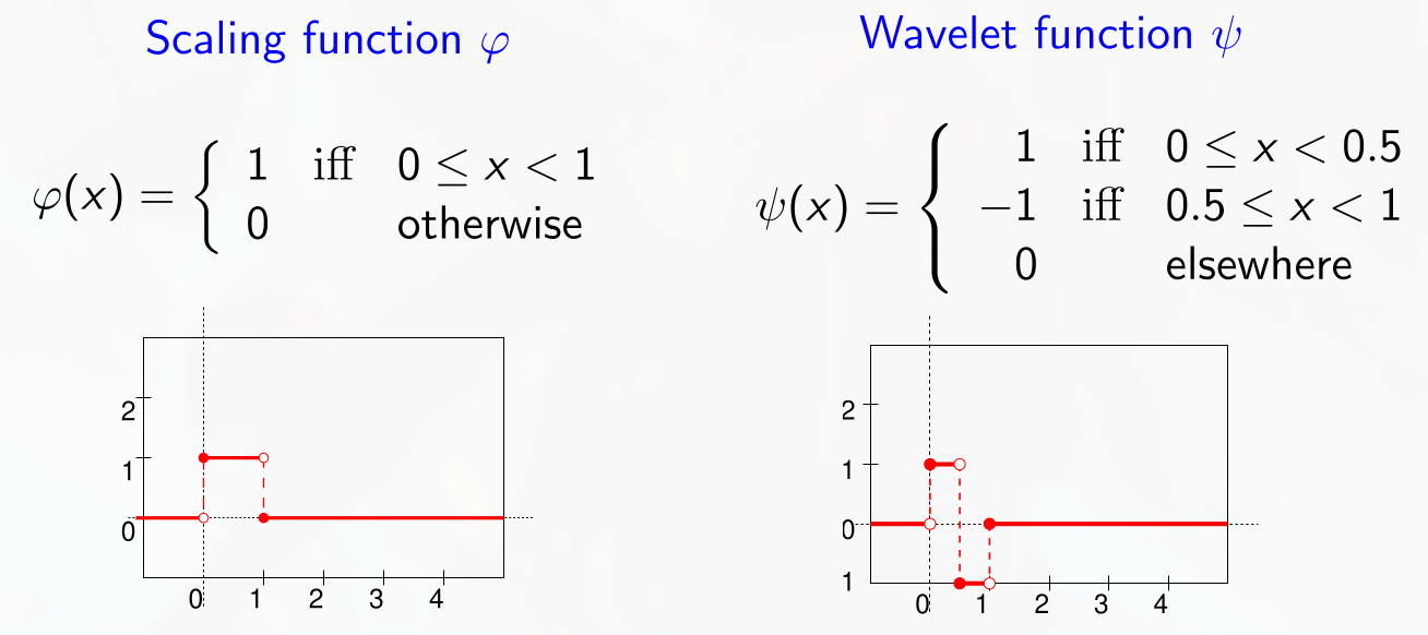
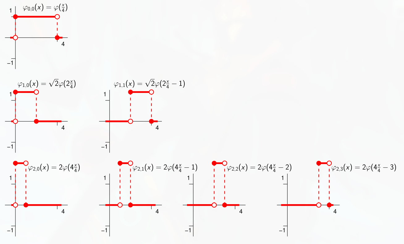
The Haar scaling and wavelet functions in DWT

We shift and scale the scaling function $φ_{j, k}$ to cover the whole signal $f$ with length $M$ :

φ_{j, k} (x) = 2^{j /2} \cdot φ (2^{j} \frac{x}{M} - k)

where:

$j$ — Scale (stretch).
$k$ — Shift along x-axis.

With growing $j$ , $φ_{j, k}$ covers a smaller fraction of the original signal range:

We shift and scale the Haar wavelet in much the same way:

ψ_{j, k} (x) = 2^{j /2} \cdot ψ (2^{j} \frac{x}{M} - k)

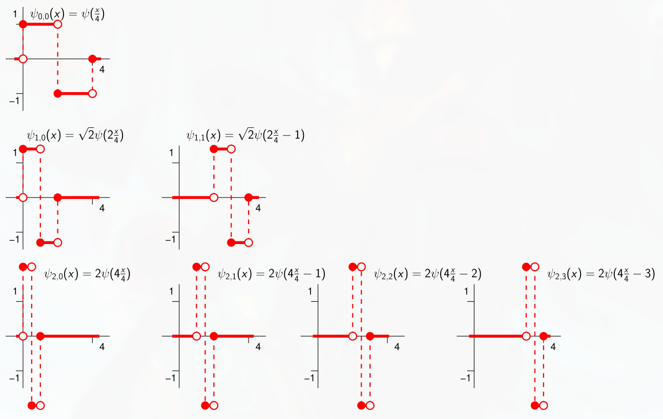Note	Notice that $φ$ is a box filter (a low-pass filter), whereas $ψ$ is a difference filter (a high-pass filter). Both functions are orthogonal to their integer shifts because their range is $⟨ 0, 1 ⟩$ .

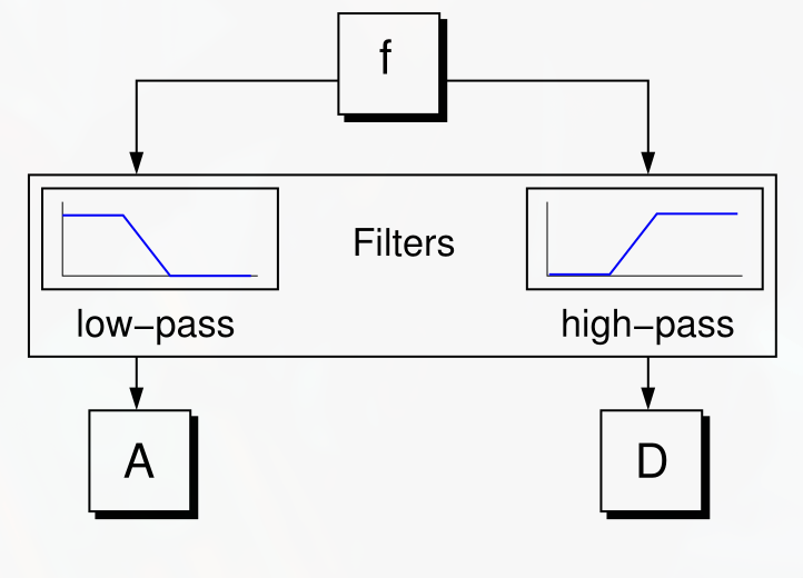
Filterbank

An array of bandpass filters that separate the original signal into multiple components, each carrying information about a sub-band.

DWT with the Haar functions

$φ_{j, k}$ and $ψ_{j, k}$ form the basis of the DWT.
$j$ controls which sub-band is analyzed; it’s the decomposition level.
- $0 \leq j < lo g_{2} (M)$ covers all frequencies.
- $0 ≪ j_{0} < lo g_{2} (M)$ focuses on high-frequencies ( $j_{0}$ is the lowest decomposition level).
$k \in {0, 1, ..., 2^{j} - 1}$ shifts the focus the k-th "fraction" of the signal being decomposed.
Haar wavelets are given explicitly. The other families are enumerated (given by a table of values).

Fast discrete wavelet transform (FastDWT)

Each step corresponds to convolution with a high-pass and low-pass decomposition filter followed by down-sampling.

It performs sub-band coding.
If it has odd length, we pad it from the right.
Has complexity $O (n)$ compared to FFT’s $O (n lo g n)$ .

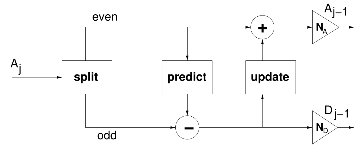
Fast lifting wavelet transform (LiftingWT)

An even faster DWT than FastDWT. The idea is the same as in FastDWT except the transition between decomposition levels is computed differently. It gets rid off the convolution and tries to "predict" the data instead. Has three broad phases:

Split into odd and even samples. (AKA the lazy wavelet)
Predict the odd samples based on the even samples and store the difference between the actual and predicted values (error) instead of the actual odd samples. (AKA dual lifting)
Update the even samples by adding the error. (AKA primal lifting)
(Normalize the output to avoid boosting the original signal.)

Compared to FastDWT, LiftingWT:

Requires less memory, since it can be computed in-place (overwriting the previous values).
Can be computed on integers only, avoiding floating-point arithmetic.

2D DWT

We use these functions:

$φ (x, y) = φ (x) \cdot φ (y)$ scaling function at row $y$ and column $x$ .
$ψ^{H} (x, y) = ψ (x) \cdot φ (y)$ intensity variations along columns.
$ψ^{V} (x, y) = φ (x) \cdot ψ (y)$ intensity variations along rows.
$ψ^{D} (x, y) = ψ (x) \cdot ψ (y)$ intensity variations along diagonals.

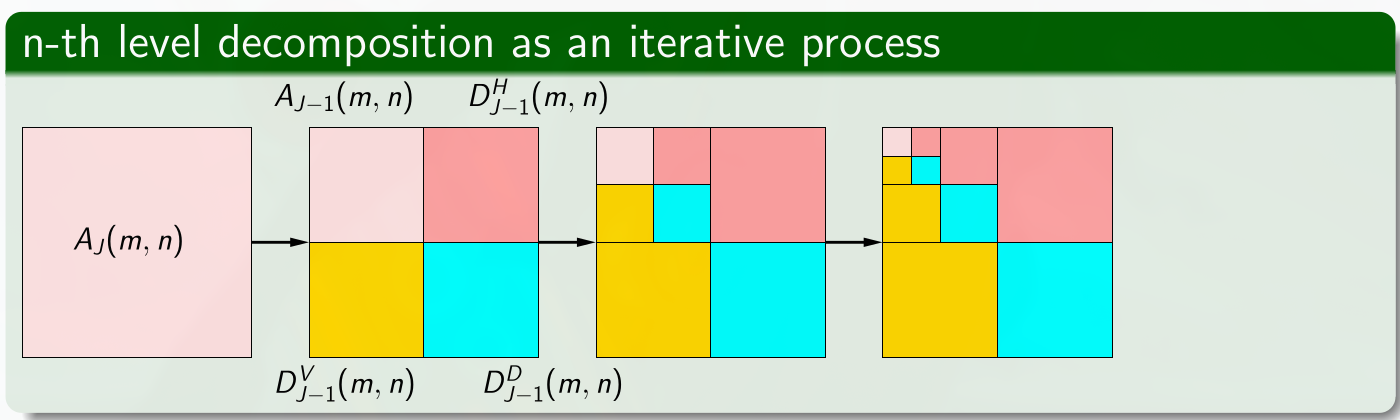
Used for edge detection, removal of high frequencies, image compression (JPEG 2000) (e.g., for fingerprint databases), image fusion (merging photos)

Questions

Explain the relationship between DFT and DCT.: DCT uses DFT under the hood. It uses some properties of DFT to remove the imaginary part of the result. As a result DCT uses some of the nice properties of DFT.
Describe the F-DCT algorithm and compute $F-DCT ([1, 6, 6, 1])$ .: See F-DCT above.

Sources

PV291
PV229
Artem Kirsanov, Wavelets: a mathematical microscope, 2022
PolyValens, A Really Friendly Guide To Wavelets