Fourier Series and Transform

Editovat

Fourier analysis

Study of how general functions (e.g., on $R$ ) can be approximated by sums of simpler (e.g., trigonometric) functions.
Fourier’s original motivation was to solve the heat equation, a partially differentiable equation.
- A partially differentiable equation (PDE) involves multiple variables and one or more of their derivatives.
- Example: I want to know what happens, when I put two rods of different temperatures into contact.

Fourier series

Fourier series (FS)

Series expansion (CZ: rozvinutí nekonečné řady) of a periodic function into a sum of basis functions.

For basis functions, it uses $sin$ and $cos$ functions with a whole number frequency.
Foundation for Fourier analysis and expansion of periodic functions in general.
Simple mathematical tool for approximation of periodic functions.
The $F (k)$ coefficients are called frequency spectrum.
Each $F (k)$ coefficient is the projection of the $k$ -th basis function onto $f$ .
It answers the question: "How important is this basis function in the grand scheme of $f$ ?"
Typically, we use a $lo g$ scale for visualization of the coefficients.

Fourier series on $π$ -periodic functions

Any $π$ -period function $f$ can be expanded in the following way:

f (x) a_{k} b_{k} = k = 0 \sum \infty (a_{k} cos (k x) + b_{k} sin (k x)) where = \frac{⟨ f ( x ) , cos ( k x )⟩}{⟨ cos ( k x ) , cos ( k x )⟩} = \frac{⟨ f ( x ) , sin ( k x )⟩}{⟨ sin ( k x ) , sin ( k x )⟩}

$k$ — frequency at which $sin$ and $cos$ oscillate
$a_{k}$ — coefficients of even parts of $f$
$b_{k}$ — coefficients of odd parts of $f$

Fourier series on L-periodic functions

Similar to $π$ -periodic functions, but we multiply $k$ by $\frac{2 π}{L}$ , where $L \in R$ :

f (x) a_{k} b_{k} = k = 0 \sum \infty (a_{k} cos (\frac{2 π}{L} k x) + b_{k} sin (\frac{2 π}{L} k x)) where = \frac{⟨ f ( x ) , cos ( \frac{2 π}{L} k x )⟩}{⟨ cos ( \frac{2 π}{L} k x ) , cos ( \frac{2 π}{L} k x )⟩} = \frac{⟨ f ( x ) , sin ( \frac{2 π}{L} k x )⟩}{⟨ sin ( \frac{2 π}{L} k x ) , sin ( \frac{2 π}{L} k x )⟩}

Complex Fourier series on $2 π$ -periodic functions

With complex numbers the formula becomes:

f (x) x F (x) = k = - \infty \sum \infty F (k) \cdot e^{ik x} where \in ⟨ - π, π ⟩ = \frac{⟨ f ( x ) , e ^{ik x} ⟩}{⟨ e ^{ik x} , e ^{ik x} ⟩}

After expanding the inner product in the above formula for $F (k)$ , we get a conversion from time to frequency:

F (k) = \frac{1}{2 π} \int_{- π}^{π} f (x) \cdot e^{- ik x} d x where k \in Z

Complex Fourier series on L-periodic functions

We multiply $k$ by $\frac{2 π}{L}$ and adjust the scaling factor and integral boundaries, where $L \in R$ :

Expansion/Frequency → Time:

f (x) = k = - \infty \sum \infty F (k) \cdot e^{- \frac{2 π}{L} ik x} where x \in ⟨ - \frac{L}{2}, \frac{L}{2} ⟩

Time → Frequency:

F (x) = \frac{1}{L} \int_{- \frac{L}{2}}^{\frac{L}{2}} f (x) \cdot e^{- \frac{2 π}{L} ik x} d x where k \in Z

Why use complex numbers in the Fourier series and Fourier transform?

They simplify the formula:
- $cos (k x) + i \cdot sin (k x) = e^{ik x}$ (Euler’s formula)
With them, FT is can be solved linearly and expressed using matrix multiplication. Without them, it’s an optimization problem that must be solved numerically.
- If we used real numbers and, for example, $sin (km - α)$ as the basis function, we would not be able to use matrix multiplication and would have to find $α$ numerically.
Complex numbers also symbolize rotation, which makes for a nice intuitive explanation (see below).

Proof of orthogonality for the Fourier series

We want to show that::

\forall j, k \in N : ⟨ e^{i x k}, e^{i x j} ⟩ = 0 if j \neq = k

Proof:

⟨ e^{i x k}, e^{i x j} ⟩ = \int_{- π}^{π} e^{i x k} \cdot \overline{e^{i x j}} d x = = \int_{- π}^{π} e^{i x (k - j)} d x = /substitute u = i x (k - j) / = \frac{1}{i ( k - j )} [e^{i (k - j) x}]_{- π}^{π} = {2 π 0 j = k j \neq = k

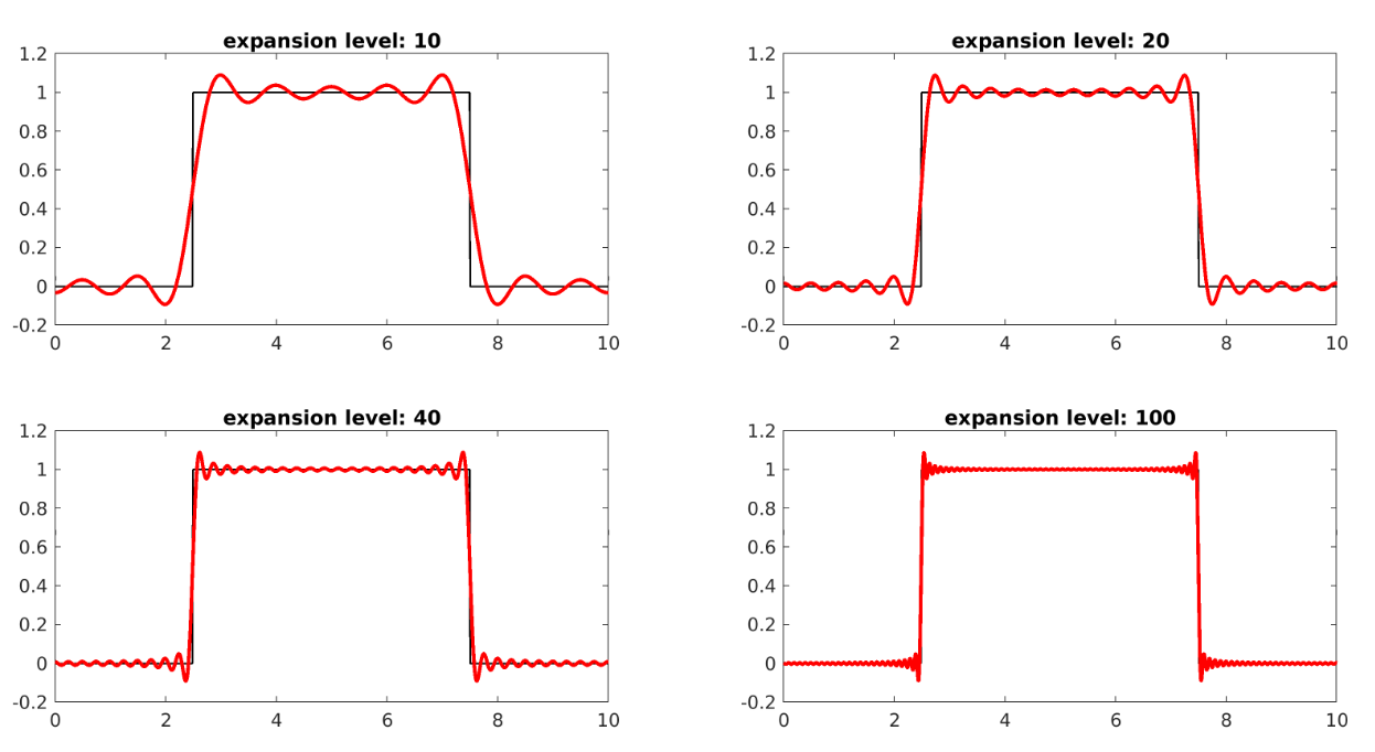
Gibbs phenomenon

Functions with discontinuities are hard to be approximated with Fourier series as $sin$ and $cos$ are both smooth.

Fourier transform

Fourier transform (FT)

A tool for frequency analysis. It decomposes a signal into a sum of sine and cosine waves of varying frequencies (and phases).

Fourier transform $F$ is a function taking a signal (a function $f$ of time) and converting it to the frequency domain (function $F$ of frequencies).

FT is a generalization of FS. It’s derived from L-periodic complex FS with $L \to \infty$ .
FS handles only periodic signal. FT handles aperiodic signal.
It’s total. Lossless. Doesn’t throw away any information. It’s invertible. A bijection. A linear mapping.

Inverse transform (frequency → time):

f (x) = \frac{1}{2 π} \int_{- \infty}^{\infty} F (ω) \cdot e^{iω x} d ω where x \in (- \infty, \infty)

Forward transform (time → frequency):

F (ω) = \int_{- \infty}^{\infty} f (x) \cdot e^{- iω x} where ω \in (- \infty, \infty)

Commonly:

F (ω) G (ω) = F (f (x)) = F (g (x))

Coefficients of the Fourier transform

Each coefficient $F (ω)$ is associated with a basis function $e^{iω x}$ oscillating at frequency $ω$ .
$F (ω) = A_{ω} \cdot e^{i φ_{ω}}$ is simply a complex number, where:
- amplitude $A_{ω}$ — strength of basis function $e^{iω x}$
- phase $φ_{ω}$ — controls the phase shift of basis function $e^{iω x}$

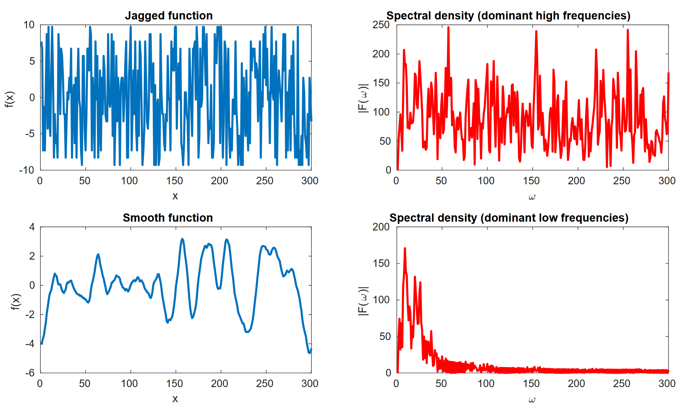
Spectral density

Plot of $F (ω)$ for $ω \in (- \infty, \infty)$ .

Function pairs in the Fourier transform

FT of the rectangle function is sinc.
FT of a Gaussian is a (different) Gaussian.

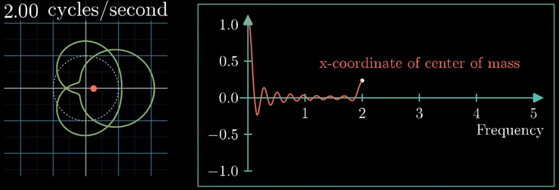
Intuitive explanation of the Fourier transform [2]

Complex numbers describe rotation, therefore multiplying $f$ by a set of complex numbers "winds $f$ up" around a circle.
Sampling this wound-up version of $f$ (whether using an integral or sum) means calculating the center of mass of the wound up version.
When the center of mass is far away from the origin, the wound-up $f$ "aligns" with itself, meaning there is a strong correlation between $f$ and the sinusoid given by the "winding" frequency.
- Except in FT, there is no division by the length of the studied interval, so it’s a "scaled center of mass". This has the effect that the more persistent a frequency is, the higher its spike.

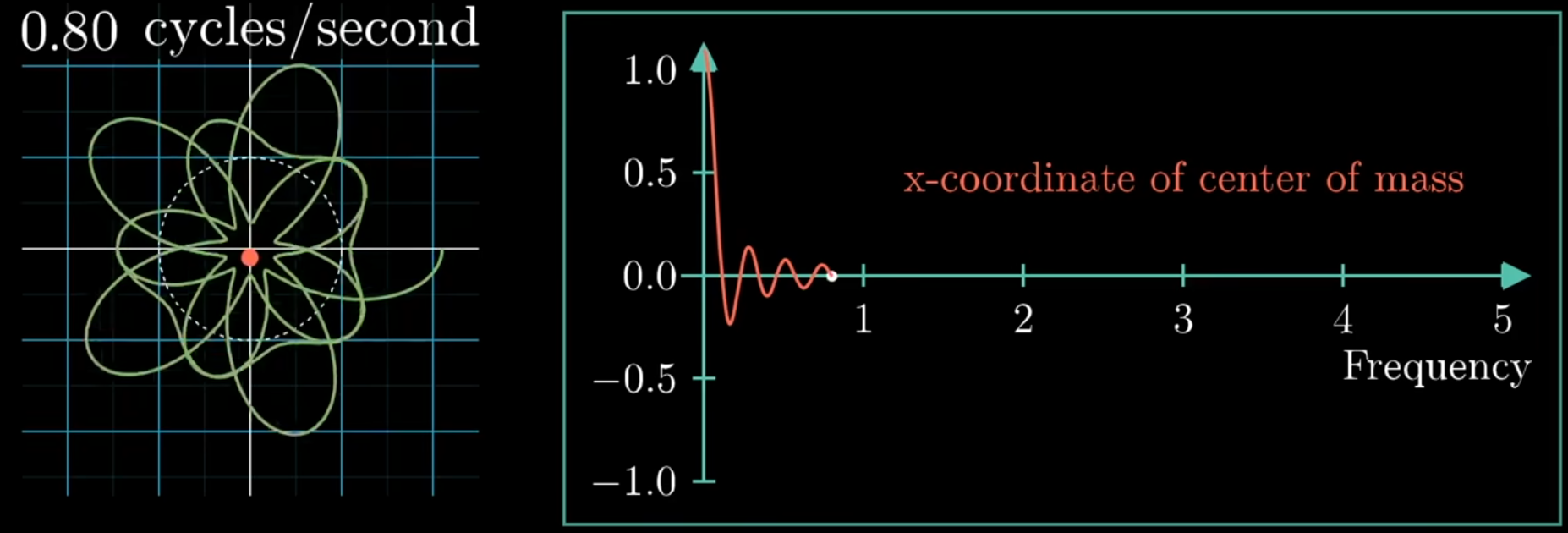
Note	The "winding" is clockwise by convention. That’s why there’s a $- i$ in the equation.

Properties of the Fourier transform

Shift affects only the phase

$F [f (x - a)] (ω) = e^{- 2 π \cdot i \cdot aω} F (ω)$
Scaling — Narrowing in the time domain causes widening in the frequency domain, and vice versa:

$F [f (a x)] (ω) = \frac{1}{∣ a ∣} F (\frac{ω}{a})$
Derivative enhances high frequencies:

$F [\frac{\partial}{\partial x} f (x)] = i \cdot ω \cdot F (ω) F [\frac{\partial}{\partial ^{2} x} f (x)] = i \cdot ω^{2} \cdot F (ω)$

Proof of scaling of FT

We want to show:

F [f (a x)] (ω) = \frac{1}{∣ a ∣} F (\frac{ω}{a})

Proof:

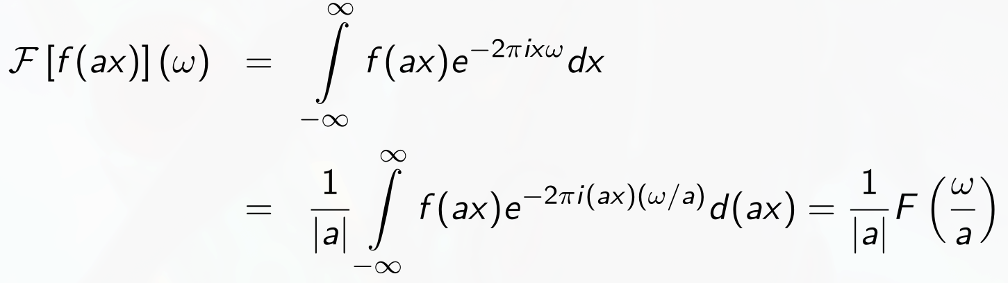Note	We solve the integral using substitution $u = a x$ . Normally, we would get a factor $\frac{1}{a}$ in front of the integral. However, we must make one case for $a > 0$ and another for $a < 0$ , which together resolve in $\frac{1}{∣ a ∣}$ .

Convolution theorem (CZ: věta o konvoluci)

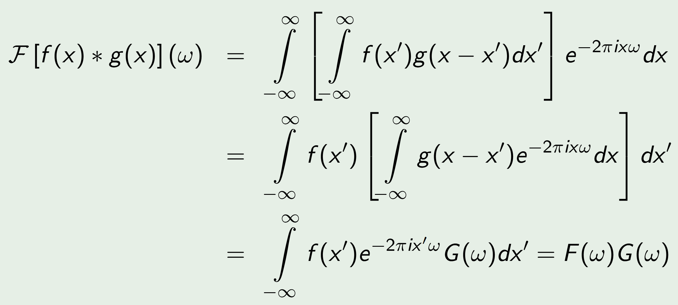
Given two signals $f$ and $g$ and their Fourier transforms $F$ and $G$ , respectively, the following holds:

$F (f * g) = F \cdot G$
$F (f \cdot g) = F * G$

where ' $*$ ' stands for a convolution and ' $\cdot$ ' for point-wise multiplication.

Proof of convolution theorem for CFT

We want to show:

F (f * g) = F \cdot G

Proof:

Discrete time Fourier Transform (DTFT)

We sample the time domain.
In other words, we turn discrete samples that are evenly-spaced in time into a continous function.
Under the Nyquist-Shannon sampling theorem we can, under certain conditions, recover the original continuous signal from the samples.
Theoretical tool used in mathematics but not in signal processing.

time → frequency:

F (ω) = k = - \infty \sum \infty f (k) \cdot e^{- iωk} where ω \in ⟨ - π, π ⟩

frequency → time:

f (k) = \frac{1}{2 π} \int_{- \infty}^{\infty} F (ω) \cdot e^{iωk} d ω where k = - \infty, ..., \infty

Discrete Fourier transform (DFT)

We obtain it from DTFT by limiting the time domain (i.e., it’s not $- \infty, ..., \infty$ anymore).
In practice, it’s finite. Mathematically, it’s infinite but periodic.

Given a discrete 1D signal $f$ of length $N$ ( $∣ f ∣ = N$ ), let $φ_{k}$ be an orthonormal basis:

φ_{k} (n) = \frac{1}{N} e^{\frac{2 πnk}{N}} = \frac{1}{N} (cos \frac{2 πnk}{N} + i sin \frac{2 πnk}{N})

where:

$n \in 0, ..., N - 1$ is the index (position)
$k \in 0, ..., N - 1$ is frequency (speed of oscillation)

Then a projection of $f$ into $φ_{k}$ basis would be:

⟨ f, φ_{k} ⟩ = n = 0 \sum N - 1 f (n) \cdot \overline{φ_{k} (n)} = n = 0 \sum N - 1 f (n) \cdot \frac{1}{N} \cdot e^{- \frac{2 π}{N} kn}

When the constant is extracted, we obtain the forward 1D DFT:

F (k) = ⟨ f, φ_{k} ⟩ = \frac{1}{N} n = 0 \sum N - 1 f (n) \cdot e^{- \frac{2 π}{N} kn}

Inverse 1D DFT (expansion):

f (n) = \frac{1}{N} k = 0 \sum N - 1 F (k) \cdot e^{\frac{2 π}{N} kn}

Note	If we define $φ_{k}$ without the $\frac{1}{N}$ , the forward transform would have no factor in the front, and the inverse would have $\frac{1}{N}$ similar to the L-periodic FS above.

Root of unity

A complex number that yields 1, when raised to some power $n$ .
An n-th root of unit is $z \in C$ where $z^{n} = 1$ .
Any integer power of an n-th root of unity is also an n-th root of unity: $(z^{k})^{n} = z^{kn} = (z^{n})^{k} = 1^{k} = 1$ .

DFT in matrix notation

Let $ψ = e^{- \frac{2 π}{N} i}$ be the Nth root of unity, then:

\overline{φ_{k} (n)} = \frac{1}{N} e^{- \frac{2 π}{N} ink} = \frac{1}{N} (e^{- \frac{2 π}{N} i})^{nk} = \frac{1}{N} ψ^{nk}

Then $A$ is the forward DFT matrix:

A = \frac{1}{N} 11111 1 ψ^{1} ψ^{2} ⋮ ψ^{N - 1} 1 ψ^{2} ψ^{2 \cdot 2} ⋮ ψ^{2 (N - 1)} \dots \dots \dots ⋱ \dots 1 ψ^{N - 1} ψ^{(N - 1) 2} ⋮ ψ^{(N - 1) (N - 1)}

and $F = A f$ , and $f = A^{- 1} F = \overline{A}^{T} F$ .

Fourier coefficients of DFT

$F (0)$ is the "direct current (DC)", "mean", or "normalizovaný součet"

$F (0) \equiv \frac{1}{N} n = 0 \sum N - 1 f (n) \cdot e^{- \frac{2 π}{N} in 0} = \frac{1}{N} n = 0 \sum N - 1 f (n)$
$F (1) \dots F (N - 1)$ are the "alternating current (AC)" terms
$F (\frac{N - 1}{2})$ corresponds to the highest frequency in $f$ (because of aliasing)

Properties of DFT

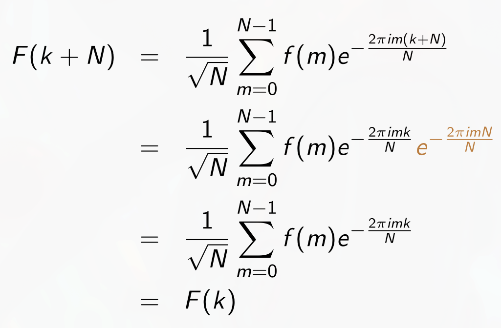
Periodicity
- We can index outside of the $N$ range and a value will be there.
- However, the input signal also seems periodic although it’s not, resulting in a "false edge".
  
  $F (k + N) = F (k)$
Oddness and evenness
- DFT of an even function missed the imaginary part ( $sin$ waves)
- DFT of an odd function missed the real part ( $cos$ waves)
Shift

$F [f (n - a)] (k) = e^{- \frac{2 π}{N} iak} F (k)$
Reciprocity — a narrow signal results in a wide frequency domain and a wide signal results in a narrow frequency domain
Hermitian symmetry

$F (- k) = \overline{F (k)}$
Linearity

$F [α f (n) + β g (n)] = α F [F (n)] + β F [g (n)]$
Convolution theorem
- It’s more effective to to a DFT followed by an IDFT than to do a convolution, but we need a long enough signal!
  
  $f * g = IDFT [DFT (f) \cdot DFT (g)] N$
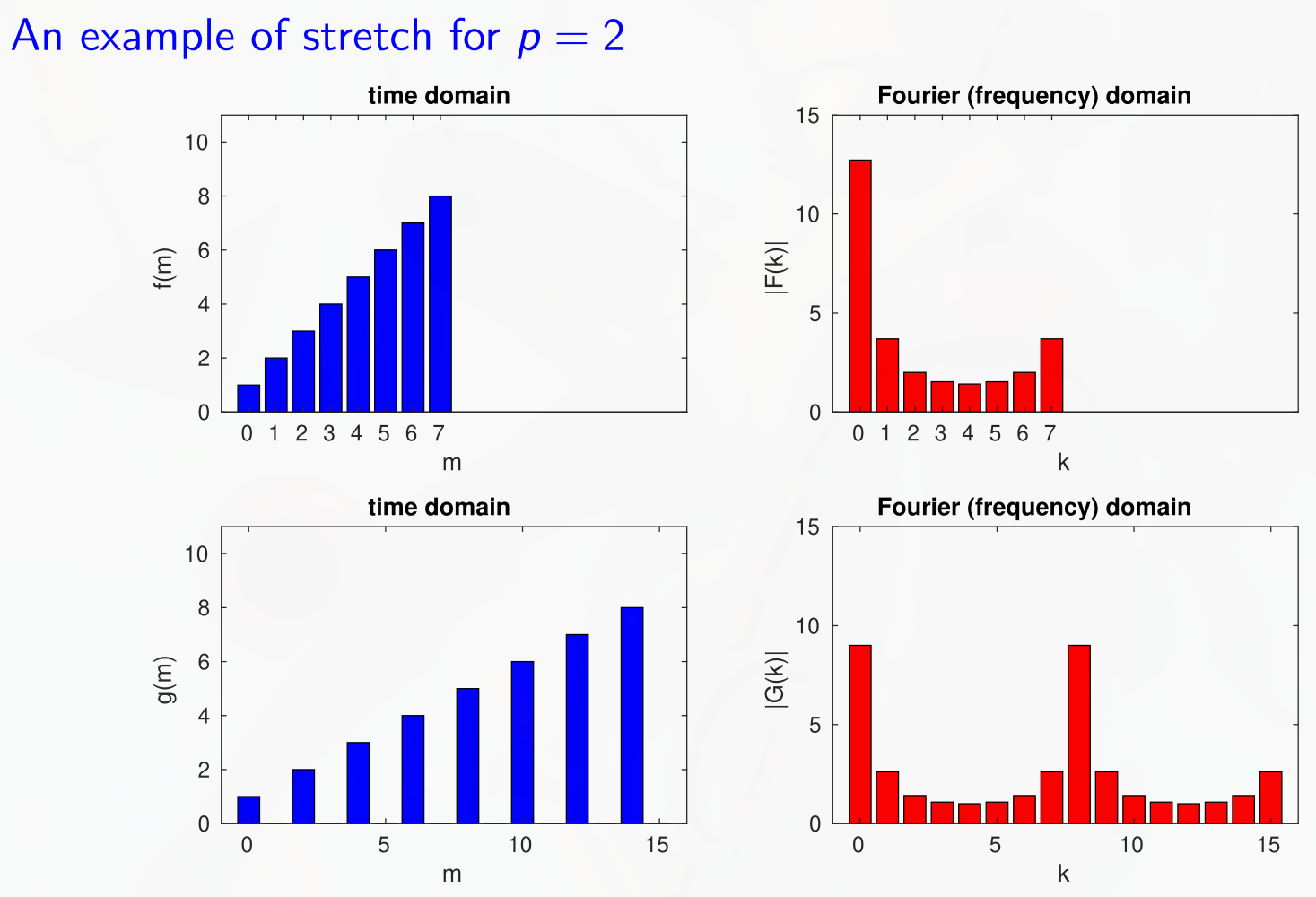
Stretch by a factor $p$ in the time domain results in $p$ -fold repetition of $F (k)$ in the frequency domain. These repetitions are dampened by $p$ .
Rayleigh theorem — Conservation of "energy".

$n \sum ∣ f (n) ∣^{2} = k \sum ∣ F (k) ∣^{2}$

Warning
Scaling doesn’t work in the discrete world. Instead, we undersample or oversample, which may result in loss of information.

Proof of periodicity of DFT

We want to show:

F (k + N) = f (k)

Proof:

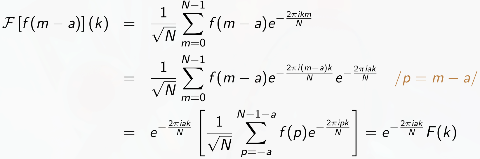
Proof of shift of DFT

We want to show:

F [f (m - a)] (k) = e^{- \frac{2 πiak}{N}} F (k)

Proof:

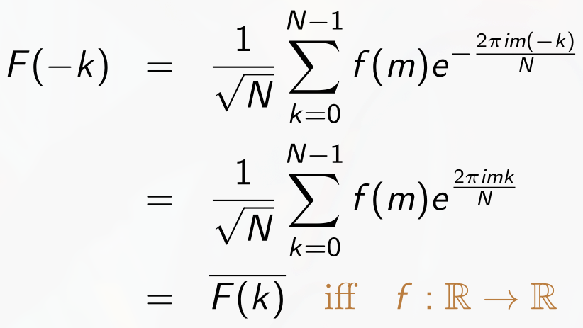
Proof of Hermitian symmetry of real signal in DFT

We want to show:

F (- k) = \overline{F (k)}

Proof:

Proof of linearity of DFT

We want to show:

F [α f (m) + β g (m)] = α F [f (m)] + β F [g (m)]

Proof:

F [α f (m) + β g (m)] (k) = \frac{1}{N} m = 0 \sum N - 1 [α f (m) + β g (m)] e^{- \frac{2 πimk}{N}} = α \frac{1}{N} m = 0 \sum N - 1 f (m) e^{\frac{2 πimk}{N}} + β \frac{1}{N} m = 0 \sum N - 1 g (m) e^{\frac{2 πimk}{N}} = α F [f (m)] (k) + β F [g (m)] (k)

Proof of the convolution theorem for DFT

We want to show:

f * g = IDFT [DFT (f) \cdot DFT (g)] N

Proof:

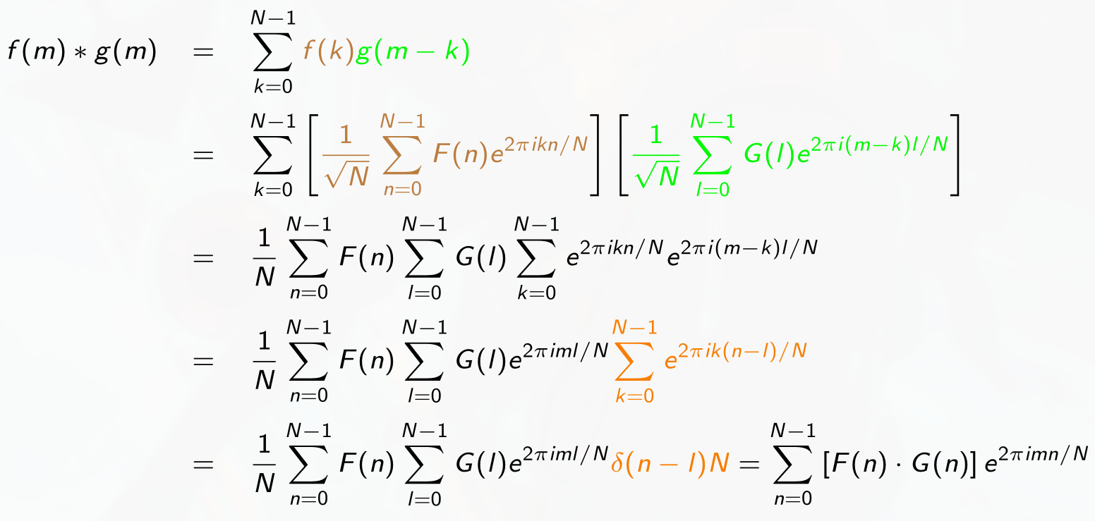
where $δ$ is Kronecker delta (not Dirac delta).

Hamming window

A solution to the "false edge" problem of DFT periodicity.
We blur the edges of the frequency domain (using a convolution).

Mixing console

Allows to limit/enhance specific ranges of frequencies.

Fast Fourier transform (FFT)

Recursive, divide and conquer.
It doesn’t really compute DFT directly, it uses its properties. Specifically, oddness & evenness, stretch, shift, and linearity:

$F (k) = \dots = F^{e} (k) + ψ^{k} F^{o} (k)$
Also that $F [x] = [x]$ . (FFT on a single sample, is just the single sample.)

Split the original $N$ -point signal ( $N = 2^{m}, m \in N$ ) into two N/2-point signals, one with all the odd samples and one with all the even samples. Run FFT recursively on each.

$F [f_{0} f_{1} f_{2} f_{3} f_{4} f_{5} f_{6} f_{7}] split into F [f_{0} f_{2} f_{4} f_{6}] = [A B C D] F [f_{1} f_{3} f_{5} f_{7}] = [P Q R S]$
Stretch the even signal to the size of the original signal. There is now a zero at every odd index. The FFT of the streched signal is the same as before, but repeated twice.

$F [f_{0} 0 f_{2} 0 f_{4} 0 f_{6} 0] = \frac{1}{2} [A B C D A B C D]$
Stretch the odd signal to the size of the original signal and shift it one to the left. The FFT of the stretched and shifted signal is the same as before, but repeated twice and phase-shifted.

$F [f_{1} 0 f_{3} 0 f_{5} 0 f_{7} 0] F [0 f_{1} 0 f_{3} 0 f_{5} 0 f_{7}] = \frac{1}{2} [P Q R S P Q R S] = \frac{1}{2} [P ψ Q ψ^{2} R ψ^{3} S ψ^{4} P ψ^{5} Q ψ^{6} R ψ^{7} S]$
Recombine the two signals (using linearity).

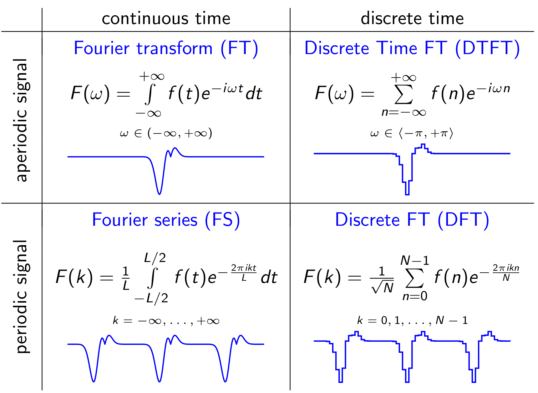
$F [f_{0} f_{1} f_{2} f_{3} f_{4} f_{5} f_{6} f_{7}] = \frac{1}{2} [(A + P) (B + ψ Q) (C + ψ^{2} R) \dots]$

1D Fourier transform formula summary

Sampling

Low-pass filter

Linear filter
Low frequencies pass through. High get suppressed.
Examples: Gaussian, Sinc, Box, Tent, B-Spline, Lanczos

High-pass filter

Linear filter
High frequences pass through. Low get suppressed.
Examples: 1st and 2nd derivatives

Sampling

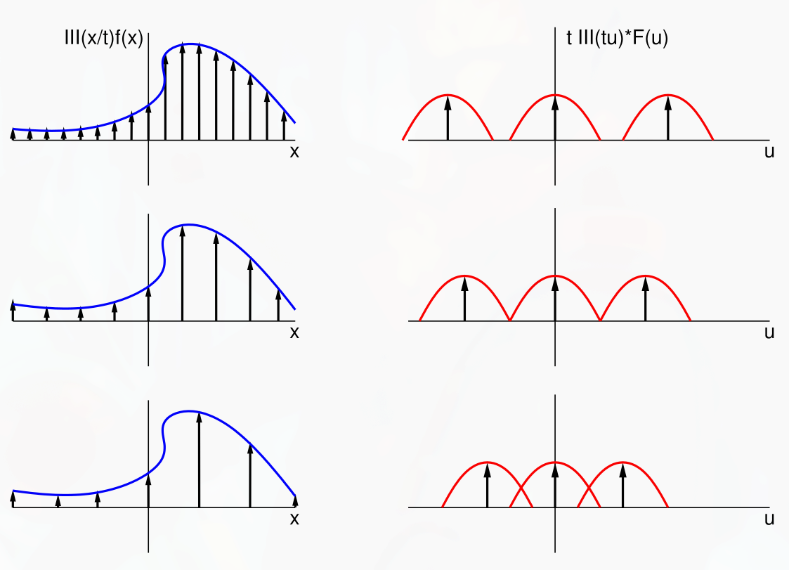
In spatial/time domain, sampling of signal $f$ is multiplication by sampling (i.e., comb) function $∣∣∣$ .
In Fourier domain, sampling is convolution of $F (f)$ and $F (∣∣∣)$ .
- Convolution with Dirac impulses, replicates $F (f)$ (much like in DTFT).
To properly sample a continuous function, it has to have an frequency upper bound, otherwise the frequency spectrum will be cut off.
The sampling frequency is limited from the lower end by us not wanting to lose information, and from the upper end by reasonability.
The comb function density must be high enough to guarantee proper sampling.

Nyquist-Shannon theorem

Exact reconstruction of a continuous signal from its samples is possible if the signal is bandlimited and the sampling frequency is greater than twice the signal maximum frequency.

Reconstruction

Reconstruction is a convolution of a discrete sequence with some low-pass filter with the objective to get the original continuous signal.

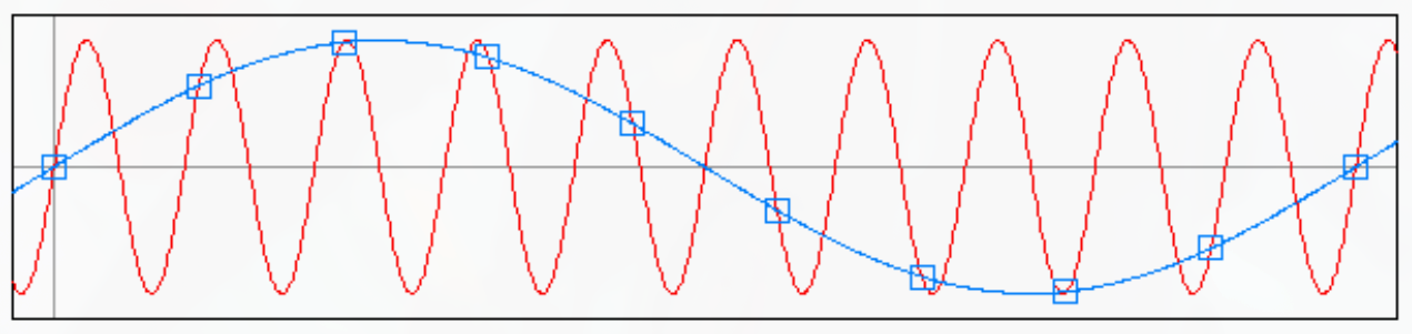
Aliasing

Phenomenon occurring when a continuous signal is sampled at a rate insufficient to capture its complete frequency content.

It happens when the Nyquist-Shannon condition is broken.
- When the sampling frequency is not high enough (e.g., wagon wheel effect).
- When the signal is not badlimited (e.g., far horizon).

Prefiltering

A solution to aliasing, where we apply a harware-based low-pass filter before sampling the continuous signal, effectivelly lowering the upper bound of its frequencies.

Resampling

Changing the sampling frequency of an already sampled signal, preferably without introducing aliasing.

Reconstruct the continuous signal from the discrete one.
Warp the domain of the continuous signal.
Prefilter the warped, continuous signal.
Sample this signal to produce a new discrete signal.

During implementation:

We don’t actually construct any continuous signal.
For each position in the resampled signal that’s being constructed, we look for the corresponding positions and their neighbors in the original signal.
Since the computation is inverted, we invert the warp ( $γ$ ) as well.

g (n) ρ (n, k) = k \sum f (k) ρ (n, k) = \int p (n - t) t (γ^{- 1} (t) - k) d t

where

$f (m)$ is the original discrete signal
$r (u)$ is the reconstruction filter
$p (x)$ is a (lowpass) prefilter
$ρ (n, k)$ is called a resampling filter
$γ (u)$ is the warping function (i.e., mapping from one coordinate system to another)
If $γ$ is affine (linear + shift), then $ρ (n, k) = p (γ^{- 1} (n) - k) * (γ^{- 1} (n) - k))$

Postfiltering/supersampling

If $γ$ is not affine, the resampling filter $ρ (n, k)$ is space-variant. In that case, we do actually have to reconstruct the continous signal from the original discrete signal, warp it, sample it at very high resolution to avoid aliasing, and the postfilter it to produce a lower resolution output signal. The convolution happens at the very end.

Fourier Transform in 2D

Fourier transform in 2D

Forward continuous:

F (u, v) = \int_{- \infty}^{\infty} \int_{- \infty}^{\infty} f (x, y) \cdot e^{- i \cdot 2 π \cdot (ux + v y)} d x d y

Inverse continuous:

f (x, y) = \int_{- \infty}^{\infty} \int_{- \infty}^{\infty} F (u, v) \cdot e^{i \cdot 2 π \cdot (ux + v y)} d u d v

Forward discrete (2D DFT) of image with $N \cdot M$ pixels:

F (u, v) = x = 0 \sum N - 1 y = 0 \sum M - 1 f (x, y) \cdot e^{- i (\frac{2 π}{N} ux + \frac{2 π}{M} v y)}

Inverse discrete (2D IDFT) of frequency domain with $N \cdot M$ values:

f (x, y) = u = 0 \sum N - 1 \frac{1}{NM} v = 0 \sum M - 1 F (u, v) \cdot e^{i (\frac{2 π}{N} ux + \frac{2 π}{M} v y)}

Frequency domain (FD) in 2D DFT

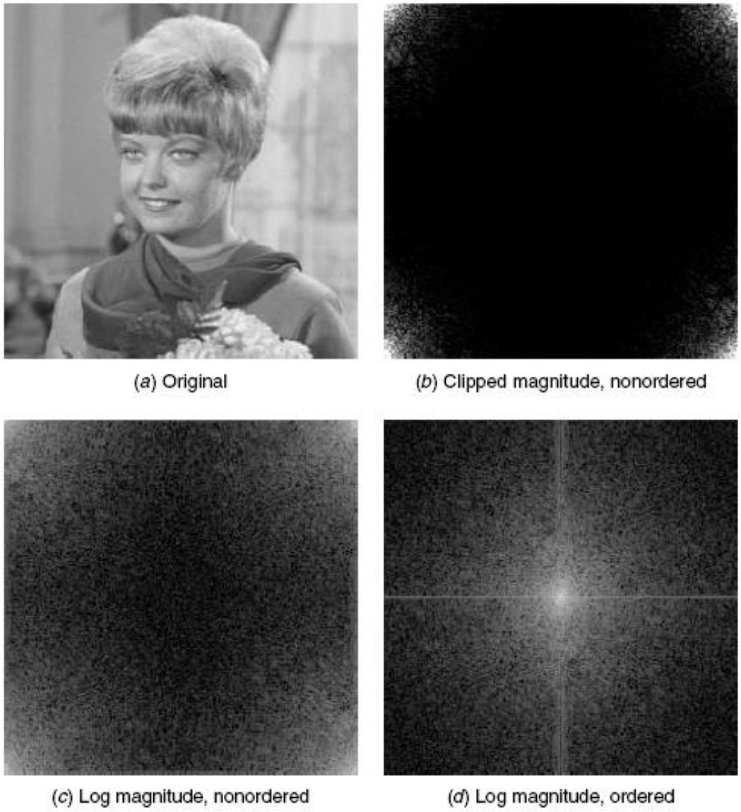
We only care about one period of FD. Thus, the FD "image" has the same size as the original.
We shift the image by $(\frac{N}{2}, \frac{M}{2})$ so that zero frequency is in the center (and not in the corner).
The FD has two components (real/imaginary, or magnitude/phase). Typically, we only display magnitude but phase still exists!
We show the FD magnitudes on a $lo g$ scale.

The phase contains what seems like noise, but it’s important for the structure (edges) of the image:

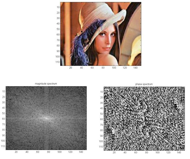
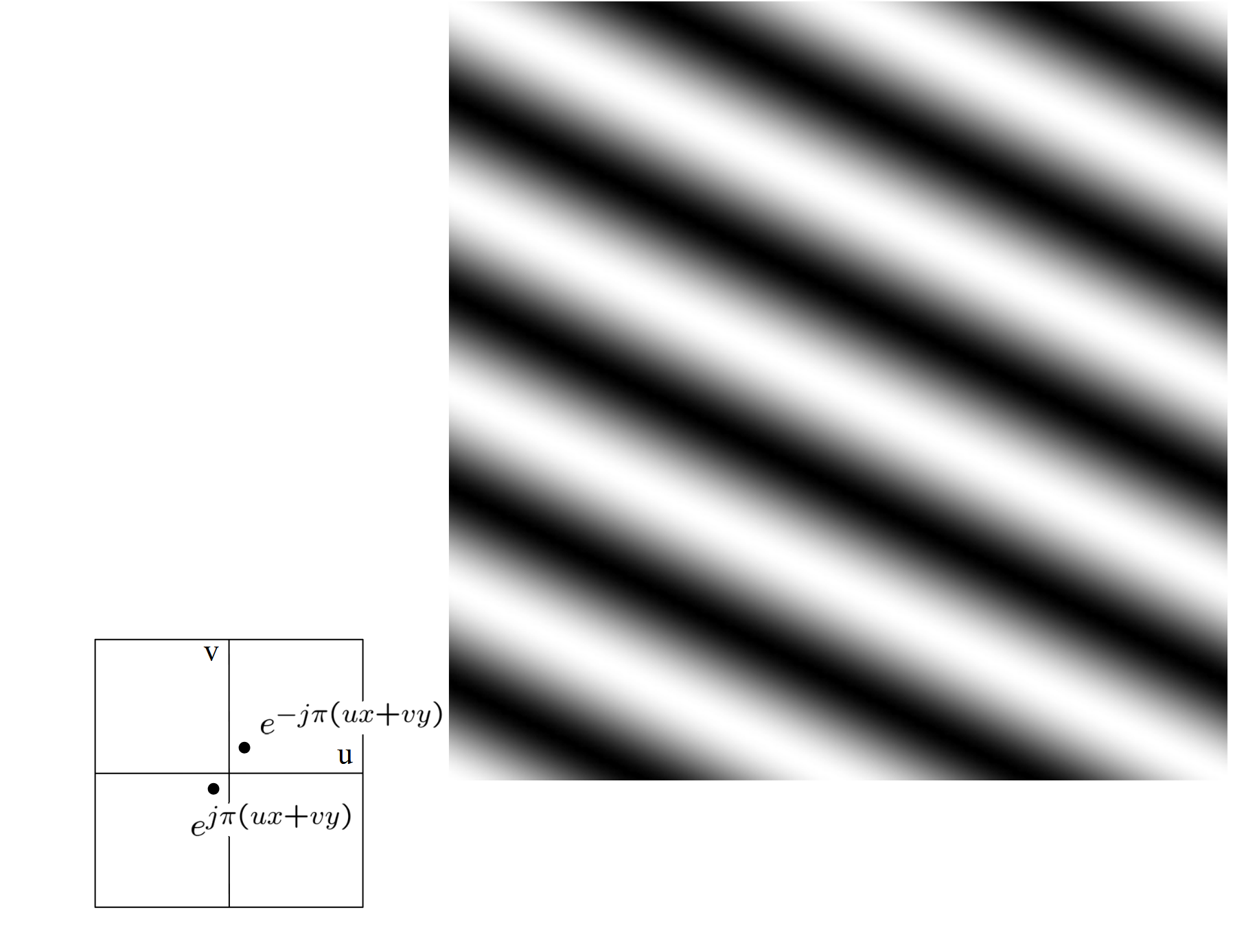
Visually, each $ω = (u, v)$ vector of FD represents a 2D sinusoidal function of $(x, y)$ . Magnitude of $ω$ is the frequency. Direction of $ω$ is the orientation of the "waves".

Questions

Explain the meaning of Fourier coefficients.

They measure the amount of correlation of a particular basis function with the expanded function.

Prove that Fourier transform is a linear mapping.

See proof of linearity for DFT above. It’s the same except there are integrals instead of sums.

Describe the spectral density plot.

A chart with two axes: x = intensity, y = frequency. Similar to a histogram.

Which frequencies dominate in the Gaussian plot?

Low frequencies, around 0.

Which operation in frequency domain corresponds to convolution in time domain?

Point-wise multiplication.

Is there ever any reason to do a convolution in the frequency domain?

Yes. If we do a convolution in the frequency domain, we duplicate the signal many times. We can use this to check if the sampling frequency is selected properly (not too low, not too high). See Sampling above.

Which frequencies are enhanced if we apply a derivative to an input signal?

High frequencies. Higher with every derivation.

Define a discrete Fourier basis function with frequency $k$ and overall length $N$ .

In FT, it would be $φ_{k} (t) = e^{ik t}$ (where $t \in R$ replaces length $N$ ), so in DFT it is $φ_{k} [n] = \frac{1}{N} \cdot e^{i \frac{2 π}{N} kn}$ where $n \in 0, ..., N - 1$ . ( $φ_{k}$ is a column vector.) $\frac{1}{N}$ is added for normalization.

Note	This is how the basis functions would appear in the inverse DFT, since that’s derived from FS. In forward FT, a complex conjugate is used because of how dot products work with complex numbers, therefore there is a negative sign in front of $i$ .

Create a matrix that can perform forward (discrete) Fourier transform for a signal of length $N = 2$ .

There is no point in having basis functions with frequency greater than $N$ , so the matrix will be N x N = 2 x 2:

[\overline{φ}_{0}^{T} \overline{φ}_{1}^{T}] = [e^{- i \frac{2 π}{2} \cdot 0 \cdot 0} e^{- i \frac{2 π}{2} \cdot 1 \cdot 0} e^{- i \frac{2 π}{2} \cdot 0 \cdot 1} e^{- i \frac{2 π}{2} \cdot 1 \cdot 1}] = [11 1 e^{- iπ}]

What is the product of the projection of an even function into a sin wave?

Zero.

Why are the wide functions in time domain transformed into their narrow counterparts in frequency domain and vice versa?

Wide functions have low frequencies, which are near the origin of the frequency domain. The wider the function, the lower the frequency, the closer to the origin of the frequency domain. And vice versa.

Compare the complexity of standard DFT and FFT.

Complexity of DFT is $O (n^{2})$ , because of the double sum.
Complexity of FFT is $O (n lo g n)$ , because of the binary-search-like approach.

What happens in Fourier domain if the signal samples are interleaved with zeros?

The values repeat because it’s periodic.

Prove that DFT is a linear mapping.

See Proof of linarity of DFT above.

Why does scaling not work in the case of DFT?

Because the discrete world is not infinitely scalable like real numbers are.

Explain the reciprocity of time and frequency domain.

Square functions in one turn to smooth in the other.
Wide turn into narrow.

Show an example of the aliasing effect.

Explain the difference between low-pass and high-pass filter.

Low-pass filter preserves low frequencies. High-pass filter preserves high frequencies.

What is a prefilter?

A low-pass filter to prevent aliasing while (re)sampling.

Give an example of $γ$ warping function.

Rotation, halving the resolution, offsetting by one pixel to the left, etc.

Fourier series

Fourier transform

Sampling

Fourier Transform in 2D

Questions

References